In this tutorial you learn how to
- use optimization criteria as objective functions or as evaluation metrics
- use our topo solvers, particularly our SIMP topo solver
Finally, we actually start performing topology optimization!
The TopoSolver class inherits all types of methods for solving TO problems. This contains the famous SIMP method, deep learning-based methods, as well as arbitrary combinations of these two.
In this chapter we start with an introduction of how our optimization pipeline works. For now, we will focus mainly on the SIMP method and we will discuss learned methods in the next tutorial.
For any topo solver we need to choose an optimization criterion, i.e., an objective function and constraints for which we want to optimize. Our library contains many criteria that can be used for evaluation or as objective functions. Generally speaking, we have two different types of criteria: supervised and unsupervised.
- Supervised criteria compare a given solution to a ground truth solution. These include for instance common loss functions like the "binary cross entropy" (BCE) as well as many commonly used evaluation criteria for semantic segmentation, like the "Intersection over Union" (IoU) and "Dice".
- Unsupervised criteria don't require a ground truth and evaluate inputs based on their intrinsic properties. They include criteria for volume, maximal stress and compliance.
We will use some of the mentioned criteria in this and in the next tutorial on trainable topo solvers.
For SIMP, we use compliance minimization with a volume constraint:
from dl4to.criteria import Compliance, VolumeConstraint

criterion = Compliance() + VolumeConstraint(max_volume_fraction=.12, threshold_fct='relu')
Compliance is a very common objective in topology optimization. It is defined as the product of external forces and displacements. The VolumeConstraint criterion compares the volume fraction -- i.e., the average voxel density -- wit a pre-defined maximum volume fraction (which in this case is 0.12). If the difference is negative (i.e., the current volume is below the maximum volume fraction) then this criterion returns 0, otherwise it returns a positive output. The thresholding can be done either via ReLU or Softplus. Both Compliance and VolumeConstraint are unsupervised criteria.
For our TO problem we choose the first sample of the disc complex SELTO dataset and we pass an FDM solver to it:
from dl4to.datasets import SELTODataset
from dl4to.pde import FDM

dataset = SELTODataset("/localdata/dl4to_dataset", name='disc_complex')
problem, gt_solution = dataset[0]
problem.pde_solver = FDM(padding_depth=0)
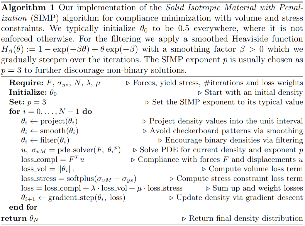
The Solid Isotropic Material with Penalization (SIMP) method is widely regarded as the most significant classical approach used in TO. SIMP employs an iterative optimization scheme to improve structural performance by adjusting voxel densities. See Algorithm 1 for a full breakdown of the steps that are part of the SIMP algorithm:

We initialize SIMP as follows, with a learning rate of 0.3:
from dl4to.topo_solvers import SIMP

simp = SIMP(
    criterion=criterion,
    binarizer_steepening_factor=1.02,
    n_iterations=70,
    lr=3e-1,
)
In order to apply a topo_solver to a problem, we can simply call it via solution = topo_solver(problem), which returns a solution object. This also works with a list of problems as input, in which case topo solver likewise returns a list of solutions.
solution = simp(problem)
Let's take a look at the solution of the SIMP algorithm:
camera_position = (0, 0.06, 0.12)
solution.plot(camera_position=camera_position,
              binary=True,
              solve_pde=True,
              display=False)


We see that the output of the SIMP algorithm returns indeed a plausible solution to the TO problem. Note that if you wish to rerun SIMP with the same simp instance, you should run simp.reset() prior to that. This is done in order to reset SIMP optimization parameters.
We can observe that the volume fraction of the SIMP solution is almost exactly 0.12:
from dl4to.criteria import VolumeFraction

volume_fraction = VolumeFraction()
volume_fraction(solution)
With DL4TO we provide an unsupervised criterion called Binariness which determines how binary the solution is. A value of $1$ means that it is fully binary, while a lower value signifies that there are more values around $0.5$. We see that our solution is almost fully binary:
from dl4to.criteria import Binariness

binariness = Binariness()
binariness(solution)
As we can observe from the above 3D plot, the von Mises stresses are well below the yield stress. The MaxStress criterion confirms this with a normalized maximal stress of less than a quarter of the maximum value of 1:
from dl4to.criteria import MaxStress

max_stress = MaxStress(normalize=True)
max_stress(solution)